Single-phase flow example

General Overview

FlowlineProSS simulates single-phase, two-phase, and three-phase flow. It performs especially well in scenarios involving export gas pipelines.

The traditional Method of Characteristics, though widely used (and sometimes misused) for single-phase flow, falls short when applied to long gas pipelines due to its oversimplified assumptions.

Gas pipeline capacity is highly sensitive to temperature, which is influenced by environmental factors such as sea currents, wind, and burial depth. These variables are often overlooked in simpler models but are crucial for accurate predictions.

To demonstrate its capabilities, FlowlineProSS includes a realistic case study of the Zeepipe export pipeline, which transports gas from the Sleipner Field in the Norwegian North Sea to Zeebrugge, Belgium. At 813 km long with a 966 mm internal diameter, Zeepipe was the world’s longest subsea gas export line when it became operational in 1993.

The Zeepipe Export Pipeline

The pipeline operator sells transport capacity through contracts ranging from daily to multi-year durations. Transport capacity is sold according to predicted transfer rates. Accurate capacity forecasting is therefore essential to optimize utilization while avoiding overselling.

The pipeline’s steel wall is encased in weight concrete to ensure stability on the seabed. As a side-effect, it also provides some thermal insulation

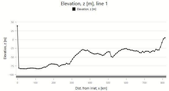
The elevation profile shows the pipeline descending from the offshore platform and following the seabed to landfall.

The inlet compressors have capacity to provide a pressure of 14.9 MPa, and the delivery pressure at the outlet end should not fall below 8.0 MPa.

Challenges involved

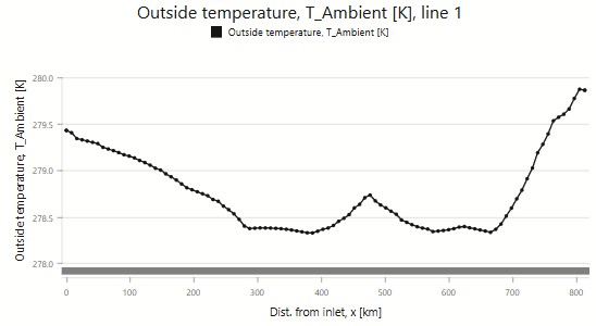
The sea and temperature varies from day to day, and that affects the gas' temperature and thereby the transport capacity. Here is a typical sea temperature forecast, used in this example:

The outlet end of the pipeline is buried. A survey some time back revealed that the rest of the line has also become partly buried:

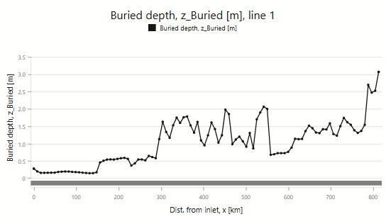
Burial depth, measured from the outer, lowest side of pipeline

The burial and part-burial has the effect of providing some added thermal insulation. Another factor to keep in mind is that the gas quality is not the same every day, so the PVT-properties must be regularly updated.

Accurate simulations must account for all of these factors - actual gas properties, dynamic actual sea temperatures, and the seabed interaction affected by the line being partly buried.

Simulating with 8 MPa Outlet Pressure

A fixed input simulation network definition with typical values for the Zeepipe system may look like this:

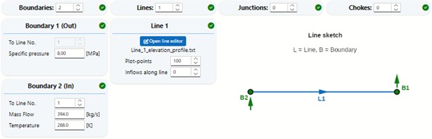
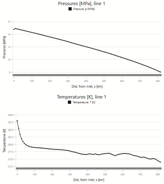
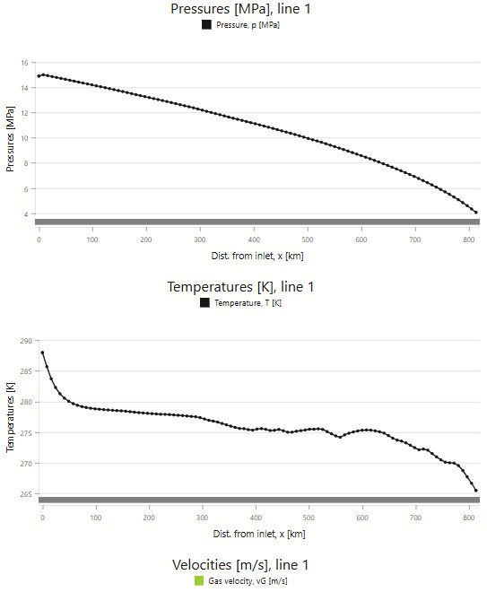
Simulations show that the inlet pressure required to achieve the given mass flow and outlet pressure is 14.9 MPa, which matches the stated maximum from the inlet compressor. This means that under these conditions, the mass flow used—394 kg/s—is the maximum steady-state flow through the line.

If simulated with FlowlineProTransient, we could demonstrate that for “short” periods (many hours or even days), gas stored in the line allows for higher mass flows than the steady-state limit. Still, the steady-state value is a useful baseline.

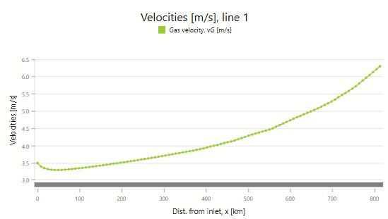
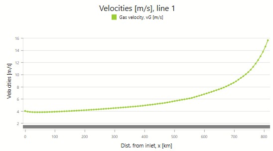
The gas velocities are very moderate—only 3.5 m/s at the inlet—and gradually increase along the line.

Gradual burial

Another interesting observation is the continuous temperature drop along the pipeline. Initially, the gas cools rapidly toward the sea temperature. But it continues cooling even beyond that, emerging at 274 K, despite the ambient temperature being 280 K.

This is due to the Joule-Thompson effect, which cools the gas as it expands. The resulting lower temperature and higher gas density slightly increase the line’s capacity— allowing a higher mass flow at the same pressure settings.

This means that gradual burial of the pipeline over time improves thermal insulation and increases capacity. Contrary to theories suggesting a “polishing effect” from gas flow along the pipe’s interior, the observed gain is clearly linked to increased burial.

Users can load the example and experiment with different temperature profiles and sea current conditions to study their impact on pipeline efficiency. In FlowlineProSS, sea temperature and current are defined as part of the elevation profile and can be easily modified.

Varying the inlet pressure

FlowlineProSS' turn-down curve calculations are most often used to determine the turndown rate in multiphase flowlines. However, they can also be applied to single-phase pipelines.

Here’s an example using 8 MPa as the minimum allowed outlet pressure:

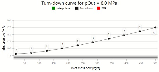
It was actually only after generating this curve that the mass flow at the inlet boundary was specified in the fixed input simulation above. From the curve, we are able to read that an inlet pressure of 14.9 MPa corresponds to approximately 394 kg/s, which is why that value was selected in the earlier simulation.

Reducing the Outlet Pressure

Contractual obligations require maintaining an outlet pressure of 8 MPa or higher. But what if we installed outlet compressors to boost pressure after the gas exits the line—allowing the outlet pressure to drop to 4 MPa?

We can explore this by generating a new "turn-down curve" for a constant 4 MPa outlet pressure:

At an inlet pressure of 14.9 MPa, the corresponding mass flow is now approximately 457 kg/s— a 16% increase compared to the 8 MPa outlet case.

A fixed input simulation with these values shows a significant increase in velocity:

The outlet velocity has increased by a factor of around 2.5. That is more than proportional to the outlet pressure reduction— but it still remains within manageable limits, not least because the pipeline carries processed, nearly particle-free gas.

This 16% boost in baseline capacity is highly significant for such an expensive pipeline. The Norwegian Minister of Petroleum and Energy stated in 2004 that the system cost NOK 23 billion, which corresponds to approximately USD 5.8 billion in 2025, after accounting for historical exchange rates and inflation.

Perhaps an outlet compressor should be considered?