Mathematical Model

General

When FlowlineProSS simulates, it solves equations that can be considered a quasi-one-dimensional version of the Navier–Stokes equations. These equations describe:

• Mass conservation: No fluid disappears as it travels through the line.
• Momentum conservation: Forces acting on the fluid—primarily pressure gradients and friction—follow Newton's second law.
• Energy conservation: Kinetic, potential, and pressure energy are balanced against energy lost as heat.

The full transient equations look like this:

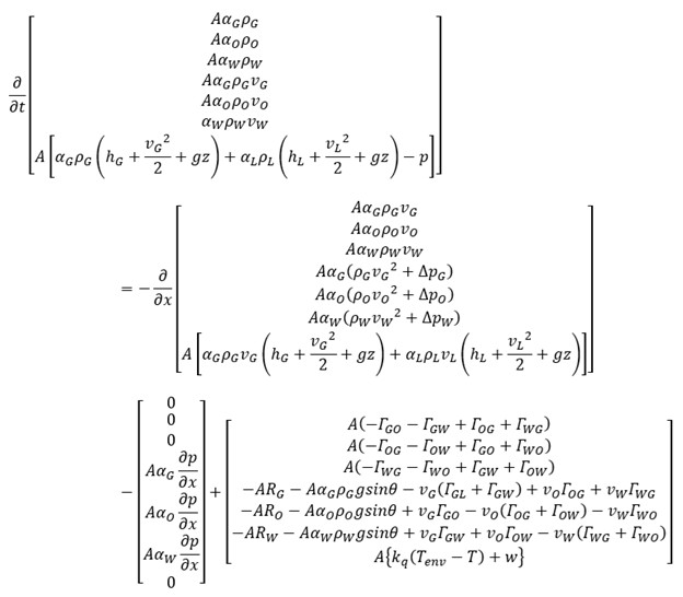
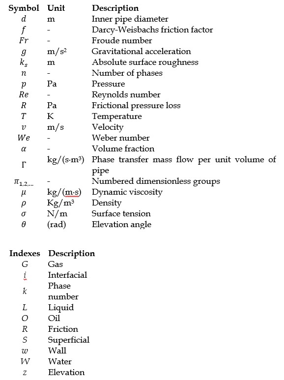
A detailed description of the symbols can be found in Pipe Flow 2’s nomenclature—the book is available via the links in the References chapter. Here, it’s worth emphasizing:

• The first three equations describe mass conservation for the gas, oil, and water phases.
• The next three describe momentum conservation for the same phases, with the friction factor R (between phases and between each phase and the pipe wall) being the most challenging component.
• The final equation describes energy conservation, including heat loss to the surroundings.
• The many Γ-terms account for phase transfer, such as gas condensing into “oil” (condensate).

Steady-state adaptation

Since a steady-state model assumes that nothing changes over time, it implies that no fluid can accumulate at any point along the line. This means the total mass flow must remain constant throughout the entire flowline.

That fact means one of the most revealing diagnostics a user can apply is to check whether the total mass flow curve is perfectly flat when plotted along the flowline (easy to do in FlowlineProSS). A flat curve confirms that the simulation respects mass conservation and that no artificial accumulation or loss is occurring. The mass flow of each phase, however, will not be flat—because phase change typically occurs.

Both FlowlineProSS and FlowlineProTransient are based on the same theoretical framework, except that for steady-state calculations, the time derivative is set to zero.

Calculating Frictions and Flow Regimes

The most challenging part of multiphase flow simulation is accurately determining flow regimes, volume fractions, and frictional losses. This task is handled by the FlowRegimeEngine (FRE), a novel module that combines well-established mechanistic models with advanced scientific methods.

Historically, multiphase flow estimates relied on empirical “rules of thumb.” Later, scientists developed a wide range of mechanistic models—many of which are detailed in Pipe Flow 2, Ref. [2]. The FRE takes this further by integrating three complementary approaches:

• Dimensional analysis
• Mechanistic models
• Neural Networks (NNs)

This triad of methods has not been fully combined in any other simulation program to date.

Dimensional Analysis

One of the key advantages of full dimensional analysis is its ability to rigorously apply physical theory to upscale laboratory measurements for full-scale flowlines. This addresses a major limitation in existing models: full-scale measurements are rare and typically limited to endpoints. As a result, extrapolation from lab data has often relied more on heuristics than scientific rigor. Dimensional analysis offers a principled and systematic alternative.

For 3-phase gas/oil/water flow, the FRE identifies 14 dimensionless groups. Combining all of them into a unified model is unprecedented—but NNs make it possible. This allows the FRE to account for all relevant parameters simultaneously, overcoming the limitations of models that focus on only a few groups per regime.

To train the NNs, FRE builds on mechanistic models with adjustable factors. These factors, not the dependent dimensionless groups themselves, are trained—resulting in faster and more accurate learning. This approach enables training with a moderate and realistic amount of data.

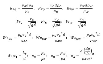
Instead of focusing solely on frictional pressure loss (π₄), the FRE can analyze other flow-dependent parameters like gas volume fraction αG. Since volume fractions are already dimensionless, αG can replace π₄ and be trained in a separate NN.

Other parameters—water, droplet, and bubble volume fractions, flow regimes, etc.—are handled similarly.

Because steady-state volume fractions remain identical when the other dimensionless groups are identical, velocities can be replaced by superficial velocities. This avoids the need for iteration during steady-state calculations.

In 2-phase gas-oil flow, water-related properties and velocity become irrelevant. This allows removal of five dimensionless groups: ReW, FrW, WeGW, WeOW, and π₃. Training a smaller NN is easier, so the 2-phase FRE is likely slightly more accurate than the 3-phase version.

Integrating Neural Networks

All FRE networks are multilayer feed-forward NNs, trained using Levenberg–Marquardt backpropagation. The number of neurons varies depending on the output type and available training data.

Flow regime classification uses a score-based system:

• Each regime (e.g., stratified, annular) receives a score based on input dimensionless groups.
• The regime with the highest score is selected.

This method works well and also provides a confidence percentage, especially near regime boundaries where scores converge.

Training the Neural Networks

Training NNs involves selecting appropriate parameters and gathering sufficient data. Even without training, the FRE performs comparably to other simulators using mechanistic models alone. Training simply enhances accuracy.

The integration of NNs with dimensionless groups enforces dimensional consistency, helping upscale lab data to industrial flowlines.

Further details are available in the IPTC article:
“Combining Dimensional Analysis and Neural Networks to Improve Flow Assurance Simulations” by Ove Bratland, Beijing, 2019, Ref. [3].

Summary of the FlowRegimeEngine

The FRE represents a novel approach to improving accuracy in multiphase pipe flow simulations. Its strength lies in merging dimensional analysis, mechanistic theory, and NN training:

• Dimensional analysis enables reliable upscaling of lab data to full-size flowlines.
• Mechanistic models provide a solid foundation, as explained in Pipe Flow 2, Ref. [2].
• Neural Networks enhance accuracy and enforce dimensional consistency.
• NNs allow integration of diverse data sources—lab results, CFD outputs, and more.
• New knowledge can be easily incorporated by retraining the NNs.
• Friction, fraction, and regime calculations are fast and iteration free—for both steady-state and transient simulations.