Getting Started
Trying Out Examples
The quickest path is to open and run a built-in example.
Click Open on the left of the top ribbon, choose Select project, and pick one.
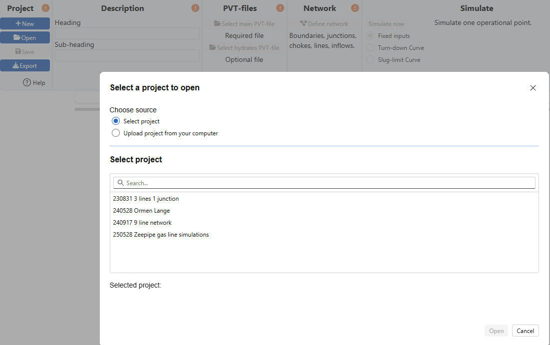
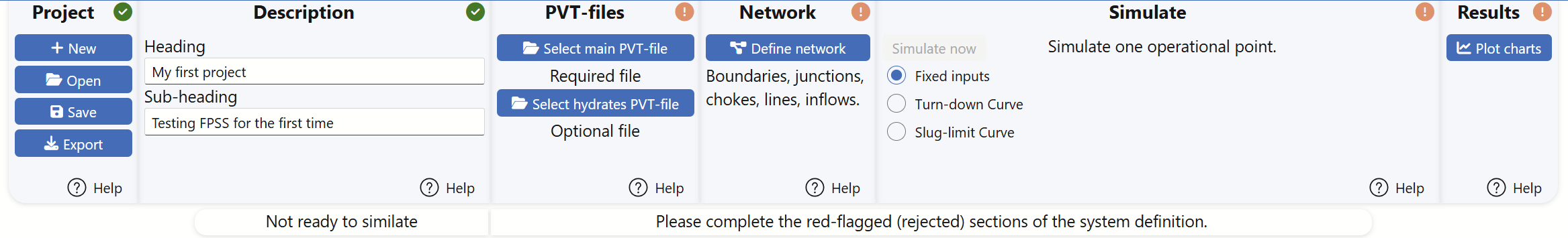
Choose Ormen Lange, and click Open. The ribbon changes like this:
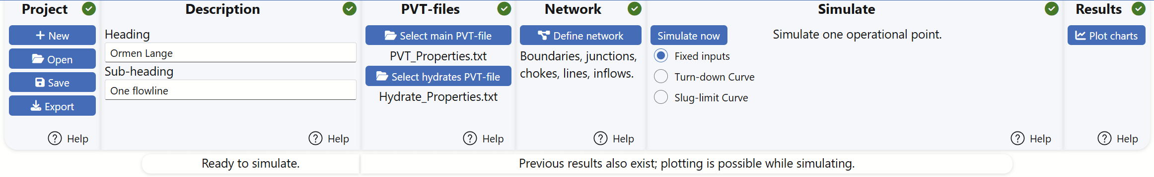
Indicators turn green when the project is fully configured and at least one simulation has completed. Hover over any button, indicator, or status text to see tooltips. Help icons open the relevant part of this manual.
Browsing one example
The Ormen Lange example includes several precomputed runs. One is a turn-down curve. To plot it:
- Click
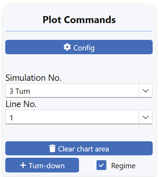
Plot charts. - In Plot Commands, choose the Turn-down curve (simulation No. 3).
- Tick Regime to overlay color-coded flow regimes along the line.
The turn-down curve looks like this:
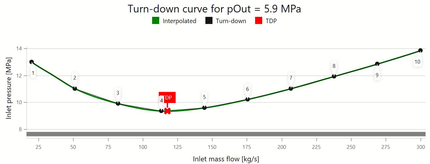
This curve uses ten mass-flow points. Point 4 is closest to the turn-down rate. Its color-coded elevation plot:
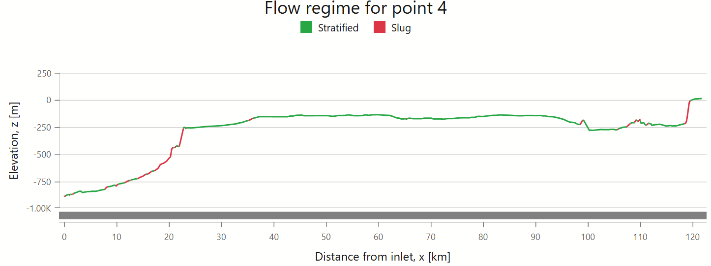
Observations near turn-down:
- Most of the line is slug-free (few red zones).
- Stratified flow (green) dominates.
- Some outlet sections still slug (red), risking slug ejection.
- Reviewing all ten points shows slugging can occur above the nominal turn-down rate.
- Turn-down curves alone are not sufficient to assess slug ejection risk.
For more detail, see Simulating and Plotting results. For geometry input, see Elevation profile.
Preparing Your Data
Define your pipeline network and fluid properties.
Fluid Data
Provide PVT data tabulated vs. pressure and temperature:
- Main PVT file (phase densities, viscosities, etc.).
- Optional Hydrate file for hydrate curves and prevention studies.
FlowlineProSS integrates with ESSS FASE PVT from December 2025 onward (included with your license). In the meantime, you can obtain PVT files from support.
Network Data
Describe connectivity and boundary conditions:
- Inlet data: mass flows and temperatures for each well
- Outlet pressure at the terminus
- Well pressures (measured or predicted) for validation
- Pipe details: diameters, materials, elevation profiles
- Seabed conditions: ambient temperature, currents
- Chokes: locations and settings
Many of these are later varied in simulations for optimization, but initial values are helpful.
Accurate seabed angles matter—small slopes near horizontal can change holdup and slugging noticeably.
Inserting Data into the Program
Starting a New Project
Follow the ribbon left-to-right. Click New and name your project folder:

Use a descriptive name (e.g., My First Project).
Uploading Fluid Data Files
- Click the two PVT buttons in the ribbon.
- Upload the Main PVT file; the orange PVT indicator turns green if valid.
- Upload the Hydrate file (optional).
If your pressures/temperatures fall outside the PVT range, the PVT indicator turns orange—you’ll need updated fluid data.
Defining the network
Click Define Network to open the network menu—most fields are self-explanatory.
A detailed walk-through is in Networks.
For a first try, leave defaults, but set Boundary 1 outlet pressure and Boundary 2 mass flow and temperature:
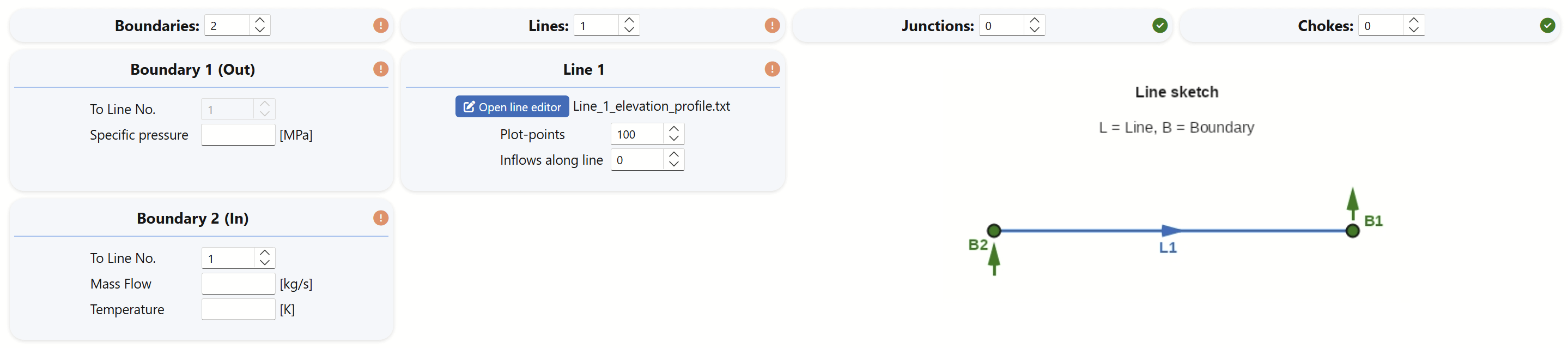
You must also click Open line editor to define the flowline and surroundings.
The editor grid shows which values go where; see Elevation profile for details.
For a minimal test, two rows (inlet and outlet) are enough—the program interpolates between them.
Simulating the system
Fixed input
When the Simulate indicator is green, you’re ready. With Fixed inputs, it simulates one operating condition with the boundary conditions specified in the Network-section. This is the simplest starting point.
Advanced alternatives
If your "system" consists of only a single line, you can also simulate turn-down and slug-limit curves—see the Simulating chapter.
Looking at results
Click Plot charts to open the plot menu.
All simulations are stored; by default, the last run is selected for plotting.
For fixed-input runs you can plot pressures, temperatures, phase fractions and mass flows, velocities, regimes, and more.
For turn-down and slug-limit curves, it is generally the curves and the corresponding flow regime plots for each point along the curves which may be plotted.
Plots can easily be copied as images or exported as underlying data (e.g., to Excel) by right-clicking on each. See the chapter Plotting results for details.