Plotting results

General

The sidebar of the plot page keeps track of all simulations, and makes it easy to plot all parameters of interest.

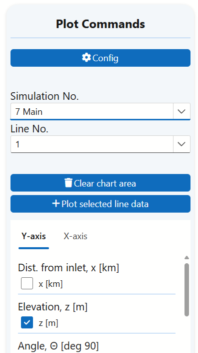
In the example shown above, there are many simulations, and any one of them may be plotted. Plot No. 7 has been selected. It is of type Main, corresponding to the fixed inputs simulation type (the first of the 3 alternatives listed by the Simulate now-button).

The Config button allows you to specify which simulations are available in the Simulation No. selector. This feature is typically used to hide simulations that, upon further review, are deemed less relevant—without permanently deleting them.

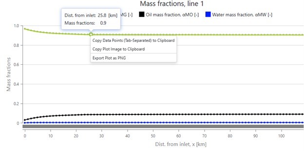
Each of the points on the plots may be investigated more thoroughly by pointing the cursor to it. At the picture below, we see that for the point the cursor points to, the x-value (distance from inlet) is 25.8 km, and the mass fraction (for the gas, which is what the green line is for) is 0.9.

At the same point, the user has right-clicked, and that brings up the copy-menu: The image itself can be copied or saved, or the underlaying data can be copied (and for instance pasted into a spreadsheet for further formatting).

Plotting fixed-conditions simulations

As an example, we focus on the 111th simulation, labeled as "Main", which is of the fixed-condition type. This simulation mode allows plotting any parameter against any other, though it is most common to use distance from the inlet x as the x-axis parameter.

Typical parameters available for plotting

• Elevation (z) along the line
• Elevation angle
• Phase densities
• Phase velocities
• Flow regimes
• And many other simulation outputs

By hovering the cursor over each parameter option, a tooltip appears with a brief explanation of its meaning.

Plot organization

Parameters are grouped by scale and relevance:

• Parameters of similar magnitude are plotted together in the same diagram.
• Parameters with differing scales are plotted in separate diagrams.
• Diagrams are stacked vertically, until removed by clicking the Clear chart area-button.

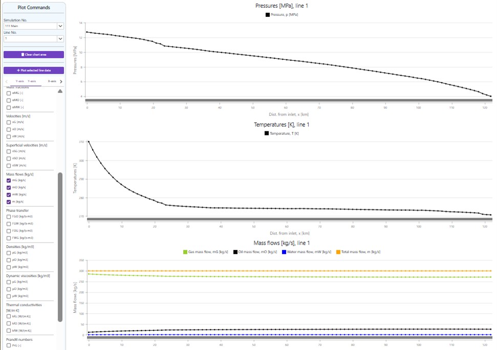
In this example, the number of plots has been limited to just three:

1. Pressure along the line.
2. Temperature along the line.
3. Mass flow rates along the line.

Make the most of browser tools

• Adjust the overall display size by holding Ctrl and scrolling the mouse wheel.
• Zoom in on individual curves for detailed inspection.
• Hover over curves to view precise point data.

The Line No. drop-down menu allows users to select different flowlines and display their plots in sequence.

Exporting Results

Simulation results can be captured in several ways:

• Right-click on a plot to copy the data, which can be pasted into spreadsheet tools like Excel.
• Save the plot as an image for documentation or reporting.
• Screenshots may also be used for quick visual capture.

Exporting and visualizing data

• Data points can be copied into a spreadsheet application like Excel, where they can be visualized in alternative formats.
• You can also simply copy the image itself and paste it into a report.

Hydrate Studies

Hydrate formation can pose serious flow assurance risks, especially in deepwater and high-pressure environments. To perform hydrate analysis effectively:

• A hydrate PVT-file must be uploaded.
• Hydrate curves can be plotted alongside pressure and temperature profiles to identify potential hydrate formation zones.

where Hydrates are most likely to form

Hydrates typically form in regions with:

• Low temperatures
• High pressures

This combination often occurs shortly downstream of the well outlet, where pressure remains near its peak, but the fluid has cooled to near seawater temperature.

Additionally, when fluids expand through subsea chokes, the Joule-Thomson effect can cause a rapid temperature drop—making these locations particularly vulnerable to hydrate formation.

Mitigation strategy

To reduce hydrate risk, it is strongly recommended to simulate scenarios using varying concentrations of MEG (Monoethylene Glycol) or other anti-hydrate additives. This can be done by uploading different PVT and hydrate files, allowing for comparison and optimization of the mitigation strategy.

Plotting turn-down curves

In this example, Simulation No. 108 represents a turn-down curve simulation. The outlet pressure was held constant at 4 MPa, while the mass flow was varied from 20 to 420 kg/s.

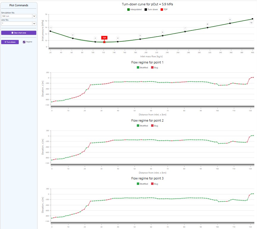
The resulting plot shows the required inlet pressure for each mass flow rate, automatically generated as a curve. A red marker highlights the minimum pressure point, located at approximately 120 kg/s.

Since the regime-selector was checked, flow regimes are also displayed along the elevation profile for each point on the turn-down curve. Only the first 3 flow regime plots have been in included in the figure above.

Observations from the Plot

• At 20 kg/s, the first plot indicates slugging at multiple locations.
• Critically, slugging is expected at the outlet, which poses operational challenges. The large liquid surges from slugs must be managed by the receiving installation.
• Increasing mass flow reduces slugging, but even at the third point—near the turn-down rate—slugging still occurs near the outlet.

Slugs behave unpredictably

Much like ocean waves, slugs can persist long enough to reach the outlet, creating potential risks for downstream equipment.

Limitations of Turn-Down Curves

This example highlights a key limitation of turn-down curves:

• They do not predict whether slugging will occur.
• They do not assess the severity or impact of slugs if they do occur.

While turn-down curves offer some early insights into flowline design and operation, they must be complemented with detailed flow regime analysis to ensure safe and reliable system performance.

Plotting slug-limit curves

As with other plot types, we begin by selecting a simulation relevant to the analysis. In this case, we use Simulation No. 110, which is a slug limit simulation. For simplicity, the corresponding slug plots for each calculated point have been omitted.

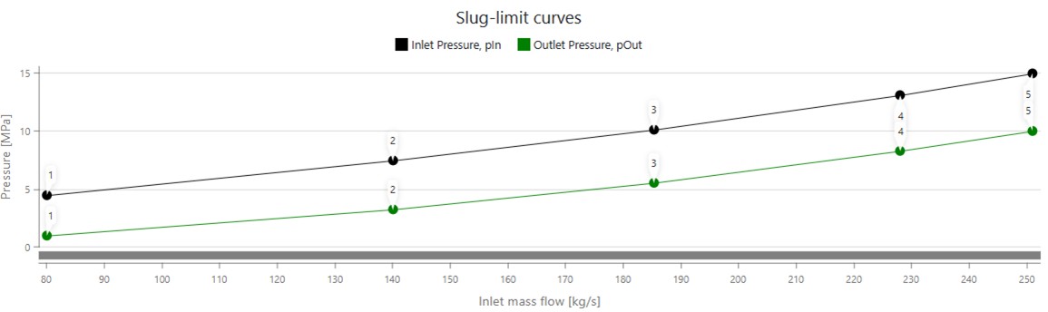
Simulation Setup

The simulation was configured to ensure that the outermost 20 km of the outlet section remains slug-free. This was specified using the range L–20 to L in the simulation menu, where L represents the point located total line length from the inlet (i.e., the outlet itself), and L–20 refers to the point 20 km upstream from the outlet. The outlet pressure was varied between 1 MPa and 10 MPa.

This analysis uses the same flowline as the turn-down curve example discussed earlier.

Understandling the curves

Typical insights from slug-limit curve analysis can be illustrated through the following example:

• To avoid slugging near the outlet, the system must operate within a mass flow range of 80 to 251 kg/s, depending on the selected outlet pressure
• The lowest outlet pressure considered (1 MPa) allows slug-free operation at the minimum mass flow of 80 kg/s
• This behavior aligns with expectations: lower outlet pressure leads to lower gas density, which in turn results in higher outlet velocities—helping suppress slug formation

These findings highlight the importance of balancing flow rate and pressure to maintain stable operation and minimize slug-related risks.

Keep an eye on erosion

• Higher flow velocities can increase the risk of erosion, particularly when outlet pressures are low.
• If high velocities are expected, assess velocity and erosion risks using the Erosion Analyzer module.

Combining turn-down and slug-limit curves

This example shows how combining several plots can be useful when investigating design and operational procedures for the different conditions at different phases of a field's lifetime.

Project Context

In a recent offshore development in Southeast Asia, FlowlineProSS was used to evaluate two alternative outlet pressure scenarios for a flowline terminating at an offshore platform.
The platform was equipped with no slug catchers and only a small inlet separator, making slug avoidance at the flowline outlet a critical concern—particularly during startup and late field life, when flow rates are typically low.

The challenges encountered in this case are representative of many offshore systems, and the findings may serve as a useful reference for analyzing similar flow assurance scenarios.

Design Considerations

A lower outlet pressure was known to increase flow velocities in the outlet section of the flowline, which helps reduce the risk of slugging. However, this approach would require installing an outlet compressor to raise the pressure to meet the inlet separator’s inlet pressure requirements. The economic feasibility of this installation was uncertain and needed to be carefully assessed.

As a first step, two outlet pressures from the flowline under consideration were:

• 8.1 MPa — without compressor
• 2.1 MPa — with new compressor installation

Objective

The goal was to determine whether the benefits of reduced slugging at lower outlet pressure justified the additional cost and complexity of installing a compressor. Multiple plots were generated to visualize flow behavior under both scenarios, helping guide the final decision:

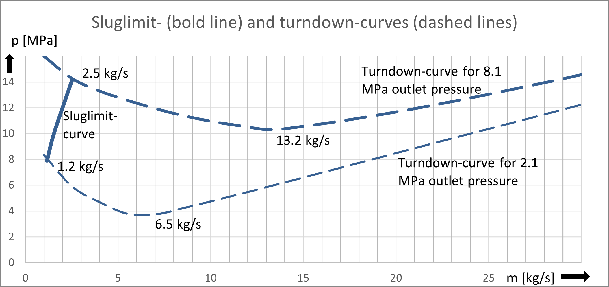
Interpreting the results

The figure above illustrates the turn-down curves for the two outlet pressures under consideration. These curves represent the minimum stable flow rates before slugging becomes a concern.

• Without a compressor, the turn-down rate is 13.2 kg/s.
• With a compressor installed, the turn-down rate improves to 6.5 kg/s.

At first glance, it might seem that production must cease once flow rates approach these thresholds, since operating below the turn-down rate is typically associated with slug formation. However, the slug-limit curve tells a different story.

Key Insights

• Both curves indicate that lower outlet pressure improves slug avoidance.
• More importantly, the slug-limit curves show that both pressure scenarios allow operation at significantly lower flow rates than the turn-down rates suggest.
• For the flowline studied here, the slug-limit curves reveals that problem-free flow can be achieved for much lower flow-rates than the turn-down rates:
  • 2.5 kg/s without compressor
  • 1.2 kg/s with compressor

Operational Implications

The system’s inherent robustness against slugging suggests that startup phases—when flow rates are temporarily low—are less problematic than turn-down curves alone might imply.
This resilience also indicates that operations can be sustained longer as production rates decline near end-of-life, without triggering severe slugging behavior.

As a result, slug-limit analysis offers a more nuanced and optimistic perspective on operational flexibility across different stages of field life.

In parallel, additional evaluations were performed using the Erosion Analyzer to assess whether increased velocities during certain phases of the field’s lifetime could pose erosion risks to the system.